The aim of Kernel Density Estimation(KDE) is:

Given a set of $$N$$ samples from a random variable, $$\mathbf{X}$$, possibly multivariate and continuous, estimate the random variables probability density function(pdf)

The univariate case

To get a rough idea how one can think about the problem, we start out with a set of samples, $$X=[x_1,x_2,…,x_N]$$, of a continuous, one-dimensional, random variable(univariate) on $$\mathbb{R}$$. To get a estimate, we assume that the pdf is constant on small intervals $$dx$$, this means our pdf is now piecewise constant and discretized. The amount of the total probability mass falling into every small interval can be written as,

$$ P_{dx} \approx f(x)dx = \frac{N_{dx}}{N}$$,

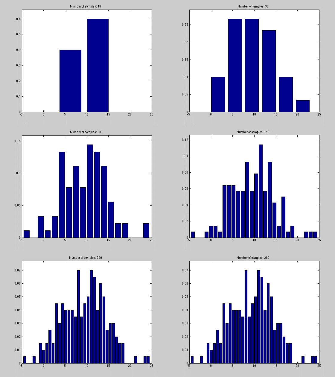
where $$N_{dx}$$ is the number of samples falling into a particular interval. What we have done, in other words, is to estimate the pdf by the normalized histogram of the samples from the random variable. In the animated gif below you can see such an estimate of a normal distributed random variable.

This estimate of $$f(x)$$ is quite blunt because of the discretization, and thus dependent on the size of $$dx$$ and the number of samples we have. We can see this in the gif above where we start out with a few set of samples and large bins, $$dx$$. As we go along, we get more samples, and can make dx finer, which results in a approximation that is quite near the original normal distributions.

The multivariate case

In the multivariate case we simply replace $$dx$$ by a volume $$dV$$ and the estimate above becomes

$$ P_{dV} \approx f(x)dV = \frac{N_{dV}}{N}. $$

We can write out the equation in units / words to get a better understanding of it:

$$ \mathrm{probability\; mass} \approx (\mathrm{probability\; mass}/\mathrm{volume})* volume = \\ (\mathrm{probability\; mass}/ \mathrm{sample}) * \mathrm{samples} $$

As we move from univariate to multivariate most of the volumes, $$dV$$, will contain few or zero samples, especially if $$dV$$ is small. This will make our discretized estimate quite jumpy.

The KDE approach

KDE approaches the discontinuity problem by introducing uncertainty (or noise) over the sample location. If there is uncertainty in the position of the sample the probability masses assigned to sample points will spread out, influencing other $$dV$$’s, giving a better and smoother estimate. Further on, since the samples now are spread out the grid or volumes estimate transforms into a sliding window estimate.

To show how this can be done we start out by specifying a kernel, $$K(u)$$, at each sample point. The kernel is equivalent to spreading out the count of a sample to the whole space. For the input to the kernel, centered at sample $$x_i$$, we write, $$ \frac{x-x_i}{dx} $$.

The input to the kernel reads as the ratio between the to-sample distance and discrectization size. We are thus feeding the kernel a value that is linear function of the to-sample distance and the grid size.

The kernel is formulated such that the following holds,

$$ \int K(u)\,du = 1 ,\; K(u) \geq 0 $$.

This looks suspiciously as a pdf, and that is essentially what it is.

Choosing the right kernel is more of a data problem than theory problem, but starting with a Gaussian kernel is always a safe bet.

$$K(\frac{x-x_i}{dx}) = \frac{1}{(2\pi dx^2)^{D/2}} e^{-\frac{1}{2}(\frac{||x-x_i||}{dx})^2}$$

$$dx$$ here becomes the variance of the kernel and restricts the sample count spread to be concentrated within the volume. Essentially, $$dx$$ controls the smoothness of the estimate, and its thus only natural that it should affect the concentration of probability mass. We can now pin down the pdf as a sum,

$$ f(x) = \frac{1}{N} \sum\limits_{i=1}^{N} K (\frac{x-x_i}{dx}) $$,

where $$K$$ is any kernel that fulfills the requirements stated above. Below is an animated gif of the behaviour of the KDE as function of the number of samples one with a fine $$dx$$

The blue dotted lines are individual kernel values (not multiplied by N), red the estimated density and magenta the actual density. The first image has a coarse grid value requiring only a few samples while the lower image has a finer grid requiring many more samples. This is one of the weaknesses of the approach since $$dx$$ is the same over the whole space and cannot be made finer where there is lot of variation and coarser when there is not. If we choose a bad average value $$dx$$ we might end up with the situation that arises in image two. Luckily there are ways to fix this but that is for another post.

A footnote, one can interpret the sum over the kernels as a mixture model where the mixture components are equal, $$1/N$$, and with the same local support. If one is familiar with the EM or variational approach to Gaussian mixture models (GMM) one can easily see the shortcomings of this static approach to density estimation as well as the simplicity and ease of implementation as compared to the GMM approach for density modeling.

For a longer more thorough explanation see density estimation by Silverman. The explanation in Bishop is also quite good.